Calculating radial distribution functions

Radial distribution functions can be calculated from one or more pymatgen Structure objects by using the vasppy.rdf.RadialDistributionFunction class.

# Create a pymatgen Structure for NaCl
from pymatgen.core import Structure, Lattice

a = 5.6402 # NaCl lattice parameter
lattice = Lattice.from_parameters(a, a, a, 90.0, 90.0, 90.0)
lattice

Lattice
    abc : 5.6402 5.6402 5.6402
 angles : 90.0 90.0 90.0
 volume : 179.42523043680802
      A : 5.6402 0.0 3.453626438275451e-16
      B : -3.453626438275451e-16 5.6402 3.453626438275451e-16
      C : 0.0 0.0 5.6402
    pbc : True True True

structure = Structure.from_spacegroup(sg='Fm-3m', lattice=lattice,
                          species=['Na', 'Cl'],
                          coords=[[0,0,0], [0.5, 0, 0]])
structure

Structure Summary
Lattice
    abc : 5.6402 5.6402 5.6402
 angles : 90.0 90.0 90.0
 volume : 179.42523043680802
      A : 5.6402 0.0 3.453626438275451e-16
      B : -3.453626438275451e-16 5.6402 3.453626438275451e-16
      C : 0.0 0.0 5.6402
    pbc : True True True
PeriodicSite: Na (0.0000, 0.0000, 0.0000) [0.0000, 0.0000, 0.0000]
PeriodicSite: Na (2.8201, 2.8201, 0.0000) [0.5000, 0.5000, 0.0000]
PeriodicSite: Na (2.8201, 0.0000, 2.8201) [0.5000, 0.0000, 0.5000]
PeriodicSite: Na (-0.0000, 2.8201, 2.8201) [0.0000, 0.5000, 0.5000]
PeriodicSite: Cl (2.8201, 0.0000, 0.0000) [0.5000, 0.0000, 0.0000]
PeriodicSite: Cl (-0.0000, 2.8201, 0.0000) [0.0000, 0.5000, 0.0000]
PeriodicSite: Cl (0.0000, 0.0000, 2.8201) [0.0000, 0.0000, 0.5000]
PeriodicSite: Cl (2.8201, 2.8201, 2.8201) [0.5000, 0.5000, 0.5000]

from vasppy.rdf import RadialDistributionFunction

The default required arguments for creating a RadialDistributionFunction object are a list of pymatgen Structure objects, and the numerical indices of the atoms (or Site objects) that we want to compute the rdf between.

indices_na = [i for i, site in enumerate(structure) if site.species_string == 'Na']
indices_cl = [i for i, site in enumerate(structure) if site.species_string == 'Cl']
print(indices_na)
print(indices_cl)

[0, 1, 2, 3]
[4, 5, 6, 7]

rdf_nana = RadialDistributionFunction(structures=[structure],
                                      indices_i=indices_na)
rdf_clcl = RadialDistributionFunction(structures=[structure],
                                      indices_i=indices_cl)

To compute a rdf between different species, we need to pass both indices_i and indices_j.

rdf_nacl = RadialDistributionFunction(structures=[structure],
                                      indices_i=indices_na, indices_j=indices_cl)

plt.plot(rdf_nana.r, rdf_nana.rdf, label='Na-Na')
plt.plot(rdf_clcl.r, rdf_clcl.rdf, label='Cl-Cl')
plt.plot(rdf_nacl.r, rdf_nacl.rdf, label='Na-Cl')
plt.xlabel(r'$r$ / Å')
plt.ylabel(r'$g(r)$')
plt.legend()
plt.show()

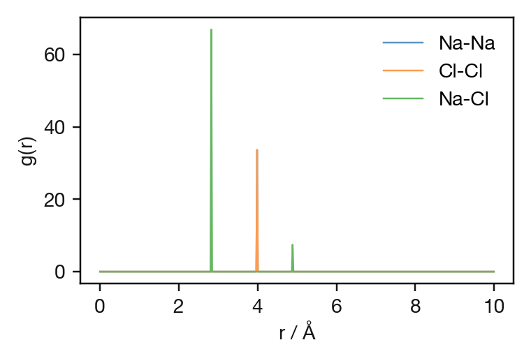
The Na and Cl sublattices are equivalent, so the Na–Na and Cl–Cl rdfs sit on top of each other.

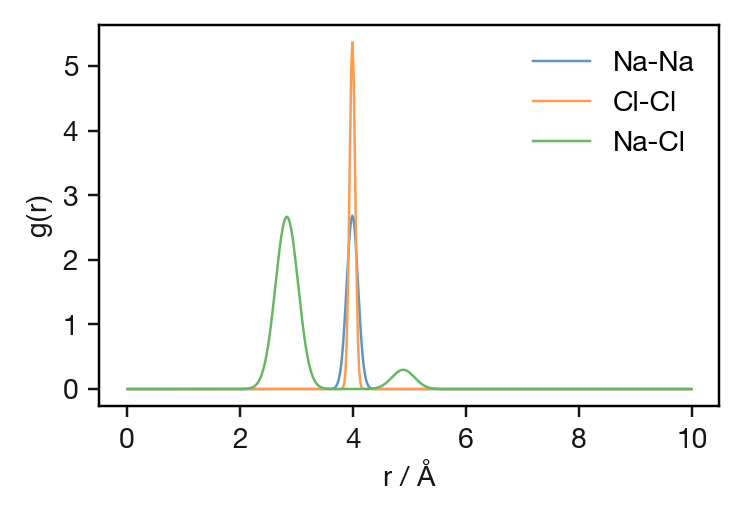
A smeared rdf can be produced using the smeared_rdf() method, which applies a Gaussian kernel to the raw rdf data. The smeared_rdf() method takes on optional argument sigma, which can be used to set the width of the Gaussian (default = 0.1)

plt.plot(rdf_nana.r, rdf_nana.smeared_rdf(), label='Na-Na') # default smearing of 0.1
plt.plot(rdf_clcl.r, rdf_clcl.smeared_rdf(sigma=0.050), label='Cl-Cl')
plt.plot(rdf_nacl.r, rdf_nacl.smeared_rdf(sigma=0.2), label='Na-Cl')
plt.xlabel(r'$r$ / Å')
plt.ylabel(r'$g(r)$')
plt.legend()
plt.show()

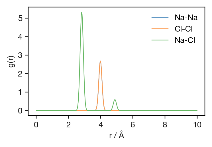
Selecting atoms by their species strings

Atom indices can also be selected by species string with the RadialDistributionFunction.from_species_strings() method:

rdf_nana = RadialDistributionFunction.from_species_strings(structures=[structure],
                                      species_i='Na', species_j='Na')
rdf_clcl = RadialDistributionFunction.from_species_strings(structures=[structure],
                                      species_i='Cl', species_j='Cl')
rdf_nacl = RadialDistributionFunction.from_species_strings(structures=[structure],
                                      species_i='Na', species_j='Cl')

plt.plot(rdf_nana.r, rdf_nana.smeared_rdf(), label='Na-Na')
plt.plot(rdf_clcl.r, rdf_clcl.smeared_rdf(), label='Cl-Cl')
plt.plot(rdf_nacl.r, rdf_nacl.smeared_rdf(), label='Na-Cl')
plt.xlabel(r'$r$ / Å')
plt.ylabel(r'$g(r)$')
plt.legend()
plt.show()

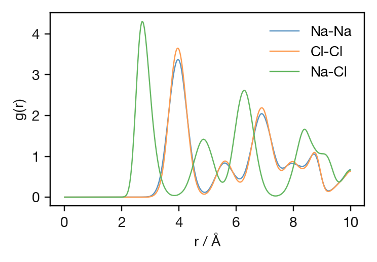
Calculating a RDF from a VASP XDATCAR

from pymatgen.io.vasp import Xdatcar

xd = Xdatcar('data/NaCl_800K_MD_XDATCAR')

rdf_nana_800K = RadialDistributionFunction.from_species_strings(structures=xd.structures,
                                                                species_i='Na', species_j='Na')
rdf_clcl_800K = RadialDistributionFunction.from_species_strings(structures=xd.structures,
                                                                species_i='Cl', species_j='Cl')
rdf_nacl_800K = RadialDistributionFunction.from_species_strings(structures=xd.structures,
                                                                species_i='Na', species_j='Cl')

plt.plot(rdf_nana_800K.r, rdf_nana_800K.smeared_rdf(), label='Na-Na')
plt.plot(rdf_clcl_800K.r, rdf_clcl_800K.smeared_rdf(), label='Cl-Cl')
plt.plot(rdf_nacl_800K.r, rdf_nacl_800K.smeared_rdf(), label='Na-Cl')
plt.xlabel(r'$r$ / Å')
plt.ylabel(r'$g(r)$')
plt.legend()
plt.show()

Weighted RDF calculations

For calculating RDFs from Monte Carlo simulation trajectories RadialDistributionFunction can be passed an optional weights argument, which takes a list of numerical weights for each structure.

rdf_nacl_mc = RadialDistributionFunction(structures=[struct_1, struct_2, struct_3],
                                         indices_i=indices_na, indices_j=indices_cl,
                                         weights=[34, 27, 146])
# structures and weights lists must be equal lengths